... which shows year-to-year changes.) However, near equlibrium, the multi-year average should be almost constant, as suggested by the curves in this plot:
Note the difference in y-axis scales between the two plots.
You should compute ice line for at least 5 values of the solar constant. Previous labs give you a head start on doing that, leaving you with at least 3 runs, most likely (depending on the choices you made for Project 2) this set:
Now run the model for two additional cases. If you have run the set above, then I suggest these two:
2. All of your runs should be sufficiently long that you can assume
you are near the equilibrium climate. Note that because the model has
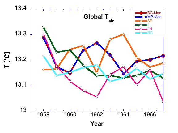
internal variability, there will always be some interannual
variability (e.g., this figure from Project 1 ...
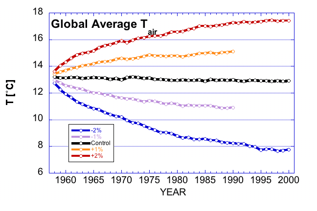
... which shows year-to-year changes.) However, near equlibrium, the
multi-year average should be almost constant, as suggested by the
curves in this plot:
Note the difference in y-axis scales between the two plots.
You will need to decide how long is "long-enough" to get acceptable 8-year averages. The figure suggest that the 2%-change runs could take some time. Discuss your simulation lengths with Prof. Gutowski and be prepared to make some estimate of how much your results might change if you ran much, much longer.
3. Once you have your 5 runs, you need to pull out some statistics. Here we are looking for the snow and ice cover. For each of your runs, each with its own "Run ID", there are two relevant output files, which give the percentage of area covered by snow and ice:
These files are in the same folder where the SRFAIRTMP file resides for each run. They also have the same format for their data. Here, however, we must be careful about using the snow and ice data because the model can have snow on top of ocean ice. (There does not appear to be any land ice designated in the model.)
We want the sum total area covered by snow and ice, recognizing that snow may be on top of ice. First consider the SNOWCOVER file. The percentage of snow covering the earth in the annual average appears in the "Global" column. Compute the 8-year average for that number.
We then need to add the additional ocean-ice percentage that is not covered by snow. The percentage of ice covered by snow appears in the "Ocean Ice" column. In the control run, it will be a number around 85%. Compute the 8-year average of the percent of ocean ice covered by snow, SNWPCT, and save the percentage of snow-free ice, (100-SNWPCT).
Now look at the OCNICECOV file. Compute the 8-year average of the "Global" ocean-ice cover. Multiply this by the percentage of snow-free ice to get the additional percentage of the globe that is covered by ice but not snow. Add that number to your snow-cover percent to get the total snow and ice cover for the globe (as a percent).
(Aside: Strictly speaking, we should compute the percentage of snow-free ice on a year-by-year basis and average that, but the interannual variability in the percentage of ice-free snow is pretty small.)
4. We want to compare our snow and ice cover area with the theory derived in class. That theory assumes that snow and ice occurs in a simple cap extending equatorward from the poles and terminating at the same latitude for all longitudes. It also assumes symmetry about the equator.
To match with the theory, we assume that the percentage of snow and ice cover is the same for each hemisphere (which is a reasonable assumption compared to observed annual averages). We also assume that the snow and ice cover is distributed like a simple polar cap. This is perhaps more reasonable in the Southern Hemisphere, were snow and ice are concentrated primarily over and around Antarctica. It is less consistent with the Northern Hemisphere snow and ice distribution, which will tend to be farther south over land, but we will assume it is an acceptable assumption.
This is where our x = sin(lat) coordinate becomes very useful. As pointed out in the lecture, dx = x2 - x1 is proportional to the area bounded by the latitudes at x1 and x2. Integrating from the equator to latitude x, the value of x is the fraction of the hemisphere's surface area between the equator and x. This is consistent with x=1 being at the pole, since the fractional area when we include all surface between the equator and the pole is then 1 (or 100%).
Another example is for latitude 30 degrees, for which x = sin(30 deg) = 0.5. The area between the equator and 30 degrees latitude is indeed one half of the surface area of the hemisphere.
Thus, we can take the fractional snow and ice cover and immediately determine the ice line. Doing this for several climates gives us an estimate of how ice line changes with solar constant.
Here is an example, taken from a simulation:
Global snow cover:  11.25%
Global ocean ice cover:  4.95%
Percentage of ocean ice with snow cover:  85.09%

Thus,
Global percentage of ocean ice with no snow:
     (1-0.8509) x 4.95 = 0.74%

Total global snow and ice cover:  11.25 + 0.74 = 11.99%
Since 11.99% of the hemisphere has snow and ice cover, then 88.01% does
not, and the ice line is at x = 0.8801
5. Compute ice line in terms of x, and plot ice line versus solar constant. For comparison with theory, normalize the solar constant by dividing your values by the control climate's value.
6. Compare your curve versus the theoretical curve presented in class for the 1D latitudinal climate model.
Go to main web page for Climate Modeling.