1-5: Carbon Cycle, Methane

Eugene S. Takle
© 1996

The accompanying table gives estimates of the carbon content of several different major ecosystems on land. For each is given its estimated land area in hectares (1 hectare is 10,000 square meters or 2.47 acres) and carbon content in units of 10¹⁵ grams ( petagrams or megatons). From this table we can see that tropical seasonal forests and tropical evergreen forests account for nearly half of the plant carbon on the planet. The tropical rain forests, of course, have received considerable attention in the scientific literature and in the public press as being particularly valuable because they contain so much of the earth's plant carbon and also because they serve as hosts for perhaps even millions of biological species, many of which have not yet even been cataloged. 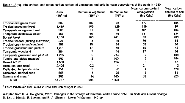Area coverage, plant carbon and net primary production for major terrestrial ecosystems. (From Takle.)

Boreal forests have carbon approximately comparable with the tropical evergreen forests, and temperate forests add somewhat smaller but significant amounts. Grasslands and pasture in temperate zones, such as native prairie in the US Midwest, contribute a relatively small amount to the total vegetation carbon total compared to the forested regions of the tropics or boreal areas. It is informative, however, to consider the amount of plant carbon per unit area in each land class (divide the values in the second column by the values in the first column to get values in the fourth column). Cultivated land in temperate zones supports only slightly less than half as much carbon per hectare as native temperate prairies. By breaking the prairie sod, the early settlers in the Midwest began the process of reducing plant carbon in the region by over 40%. This is, of course, in addition to the accompanying deforestation that took place at the prairie margins. It might be tempting to argue that a lush Iowa cornfield with 30,000 or more plants per acre would have more plant carbon than native prairie vegetation, but the data suggest otherwise.

The next column lists carbon in soils. Boreal forests and tundra and alpine meadow contribute almost identical amounts to the total planetary soil carbon. Expansive temperate grasslands and pasture contribute nearly as much total soil carbon as the boreal forest soils, but somewhat less on a per-hectare basis. The per-hectare values of the fourth and fifth columns can be expressed in kilograms per square meter by dividing these numbers by 10. Hence, tropical evergreen forests have about 17.7 kilograms per square meter of carbon in the vegetation and temperate grassland or pasture have about 0.7 kilogram per square meter. The most notable entry in this column is the enormous carbon density in soils of swamps and marshes, being over 2 1/2 times as much as the next largest entry. Tillage of soil increases microbe activity in the soil and leads to more rapid conversion of soil carbon to CO₂. The small marshes and wetlands, known as prairie potholes, that once covered the Iowa, Dakota, and southern Canada landscape were rich in soil carbon as suggested by the carbon table. Draining and cultivating these regions has resulted in the loss of significant amounts of soil carbon. One of the benefits of modern minimum-tillage and no-tillage practices is that they increase amounts of carbon that are stored in the soil.

The next table shows changes in carbon reserves for each land-use category between 1850 and 1980. In this table, positive numbers indicate a decrease in the carbon content in that particular land use category. Note that some areas show an increase in total carbon because the area of this category has increased and not because the carbon per unit area has increased. For example, cultivated lands in temperate zones have doubled their carbon content between 1850 and 1980, but this is due to a doubling of the area in this land classification. The amount of carbon per unit area in this land-use type has been essentially constant. 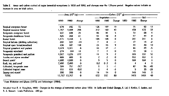Area coverage, plant carbon and net primary production for major terrestrial ecosystems in 1850 and 1980. (From Takle.)

Agricultural and forestry management practices can have a significant effect on the earth's global carbon cycle. Soil tillage practices, crop choices, and plantation and forestry management practices all impact the global carbon cycle. High latitude continental areas have vast boreal forests and frozen tundra that store carbon for longer periods of time. Many biological and physical processes depend on temperature: higher temperatures tend to accelerate these processes. For example, cooking food speeds up the physical transformation processes. In tropical areas where the temperature is high but moisture is not limiting, growth and decay processes occur very rapidly, whereas at high latitudes and high altitudes (mountainous areas) they proceed very slowly. Disturbances that occur in areas of where transformations proceed slowly take much longer to recover than in warmer climates.

Agriculture soils have lost about a third of their native carbon. Agriculture, by use of alternative tillage practices and also by eliminating excessive use of nitrogen fertilizers, may help to reduce atmospheric carbon dioxide by allowing more carbon to be stored in the soil. Nitrogen fertilizers stimulate soil processes and accelerate the transformation of soil carbon to carbon dioxide: reducing excessive use of nitrogen fertilizer reduces the amount of soil carbon lost to the atmosphere.

Carbon dioxide is a friendly gas: at atmospheric concentrations, even double the present amount, it is not harmful to humans, since it is odorless, colorless, and does not react in the human body. And plants grow more vigorously in enriched CO₂ environments, so why do we raise the concern about its increase? A significant characteristic of carbon dioxide is that it has a very long lifetime in the atmosphere. An accompanying graph shows atmospheric concentration excess as a function of time. This graph provides an answer to the following question: If we put one extra kilogram of carbon dioxide into the atmosphere, how long would it stay there? This curves shows that the atmospheric loss occurs very slowly. It takes about 60 years for half of the initial kilogram to be cycled out of the atmosphere and about 200 years to lose two-thirds of the initial amount. The lifetime of carbon dioxide in the atmosphere is obviously very long. This means that large amounts of carbon dioxide presently being put into the atmosphere by burning fossil fuels and deforestation will, on average, be around for many decades. 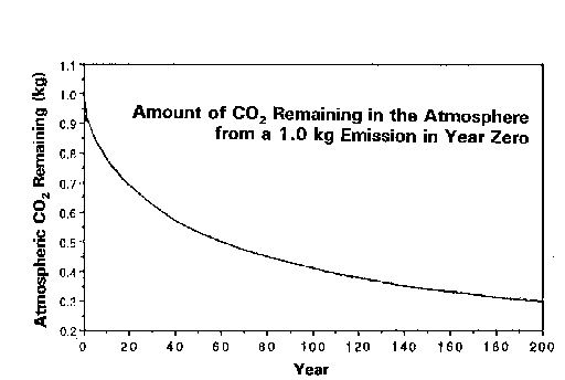Atmospheric CO₂ concentration excess as a function of time. Houghton, J.T., G.J. Jenkins, J.J. Ephraums, eds, 1990: 1990 Intergovernment Panel on Climate Change, Cambridge University Press, 364 pp.

We have identified numerous natural processes that put significant amounts of carbon dioxide into the atmosphere, much larger amounts that are contributed by burning fossil fuels or deforestation. And the uncertainty in the magnitudes of these natural sources is large, perhaps much larger than the amounts we attribute to anthropogenic sources. It is then tempting to attribute the increase to some error in our estimate of natural sources and not blame humans.

The diagram to the right shows convincing evidence that the source of much of the increase in carbon in the atmosphere is fossil fuels. Carbon has three isotopes, C¹², C¹³, and C¹⁴. Carbon 12 is the most abundant, and C¹³ and C¹⁴ are produced from C¹² in the biosphere by cosmic radiation. Once produced, the C¹³ or C¹⁴ will slowly decay back to C¹². Fossil fuels represent carbon that has been removed from the biosphere for centuries and buried under the surface of the earth where it is shielded from cosmic radiation so the C¹³ and C¹⁴ of such carbon stores have had a long time to decay back to C¹² without production of new amounts of C¹³ and C¹⁴. Therefore, fossil fuels are almost pure C¹². Combustion of fossil fuels then adds C¹² to the atmosphere but not C¹³ or C¹⁴. This means that the relative amount of C¹³ and C¹⁴ should decrease as the level of C¹² is increased. The accompanying graph shows measurements of the partial fraction of C¹⁴ in the atmosphere over the last 130 years. The data clearly show a decrease in the relative abundance of C¹⁴ during the last few decades. These data provide strong evidence implicating fossil fuels as a major contributor to the increase in atmospheric carbon dioxide. The data for C¹³ provide additional confirming evidence. 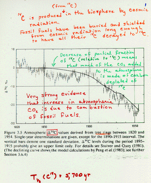Atmospheric changes in carbon 14 values derived from tree rings between 1820-1954. (Source unknown.)

The fate of carbon dioxide put into the atmosphere by burning fossil fuels can be summarized as shown in the next figure which shows the number of petagrams of carbon per year taken up by the ocean and atmosphere and ocean together between 1800 and 1990. The difference in these two curves, labeled as the "residual", is the estimated amount that must be accounted for by changes in vegetation uptake and changes in land use (e.g., deforestation, carbon or carbon-sequestering capability lost due to urbanization). The figure on the right gives the best estimate of the amount due to land use. The remainder, labeled "missing sink", suggests that there is some unaccounted-for loss of carbon from the atmosphere/ocean system. Speculation is that the boreal forest or high-latitude oceans may be responsible, but more data are needed to confirm the identity of the missing sink. 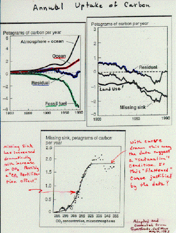Annual uptake of Carbon. (Adapted and corrected from Sarmiento, J. L., 1993: Ocean and Carbon Cycle. C & E News, May 31.)

We've looked at atmospheric carbon dioxide from the past up to the present, and now it might be informative for us to look to the future. Anthropogenic emissions of carbon dioxide to the atmosphere in the future, which occur mainly due to burning of fossil fuels, are very closely tied to economic development. Strong economic activity in developed countries and modernization of developing countries both relate closely to the production of electrical energy, use of fossil-fuel burning machines, and the use of cement. These agents of growth all produce carbon dioxide as byproducts. Presently the anthropogenic production of carbon dioxide increases about 2% per year. We can use different economic growth rates to project future anthropogenic production of carbon dioxide, as is shown in the next plot. Here it can be seen that by continuing on our present rate of growth, atmospheric carbon dioxide levels will reach 600 ppm by about 2050. Reducing our growth in production to zero (keeping emissions constant at current levels) reduces the level to 440 ppm by 2050. If our goal were to limit atmospheric levels to less than 400 ppm, we would have to reduce emissions by 2% per year. If we turned off all fossil-fuel burning power plants, stopped using automobiles, and eliminated all other anthropogenic emissions, the atmospheric carbon dioxide concentration would return to about the 1980 level by 2050. 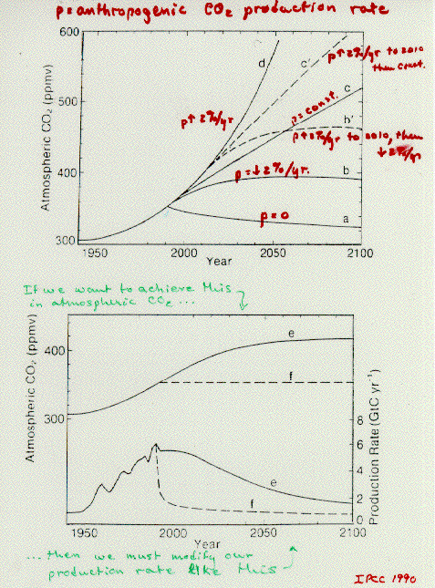Anthropogenic CO₂ production rate. Houghton, J.T., G.J. Jenkins, J.J. Ephraums, eds, 1990: 1990 Intergovernment Panel on Climate Change, Cambridge University Press, 364 pp.

This figure reveals the dilemma that we face if we seek to limit the growth of atmospheric carbon dioxide. We seem destined to have a very high level of carbon dioxide in the earth's atmosphere, compared with levels of the last 160,000 years, by the middle of the next century.

Let's briefly summarize what we have learned about the carbon cycle to this point. During the period of 1860-1994 there has been about 241 gigatons of carbon emitted to the atmosphere by fossil fuel combustion, and the rate in 1990 was 6.0 gigatons of carbon into the atmosphere due to deforestation, and the present rate is about 1.6 gigatons per year. Apparently deforestation is on the increase again in South America because of the renewed demand for farm land. Atmospheric carbon dioxide concentrations have increased from about 275 ppm in the middle of the last century to the present value of about 360 ppm or slightly more in 1996. We understand the basic features of the carbon cycle quite well. It is possible to construct quantitative models to use as a guide in projecting the CO₂ concentrations. The uncertainties of the projections of likely future CO₂ changes on the basis of a given emission scenario are considerably less than those of the emission scenarios themselves. We cannot project our economic growth very well, but if we could, we probably could project our CO₂ levels quite accurately. It will require some reduction in emissions growth rate to keep from doubling our atmospheric carbon dioxide level before the middle of the next century.

Methane is another atmospheric constituent whose concentration has increased in recent years. Methane is also a greenhouse gas that is about twenty times as effective on a molecule for molecule basis as is CO₂. One methane molecule will absorb 20 times as much infrared radiation as CO₂. Its lifetime is much shorter than carbon dioxide, however, so this partially compensates for its higher absorption.

Actually, methane is the most rapidly increasing greenhouse gas. The first plot below shows the present concentration of methane, in parts per million by volume (ppm), to be about 1.7 ppm. Sometimes methane concentration is given in parts per billion by volume (ppb), and then would have a value of 1700 ppb. The numerical values show that methane is much less abundant than carbon dioxide which has a present concentration of about 360 ppm. However, the curve shows that the concentration is increasing at about 1% per year. If we look at a longer term, as shown in the second graph below, we see that concentrations have increased substantially since the Industrial Revolution. Estimate of atmospheric methane from a thousand years ago suggest values around 0.7 ppm (700 ppb) which were constant until about the late 1700s. Since that time, concentrations have more than doubled. If we examine the Antarctic ice core data going back 160,000 years, we see that methane levels fluctuated between about 300 parts per billion and 700 parts per billion until the Industrial Revolution when it began its climb to near 1700 parts per billion.

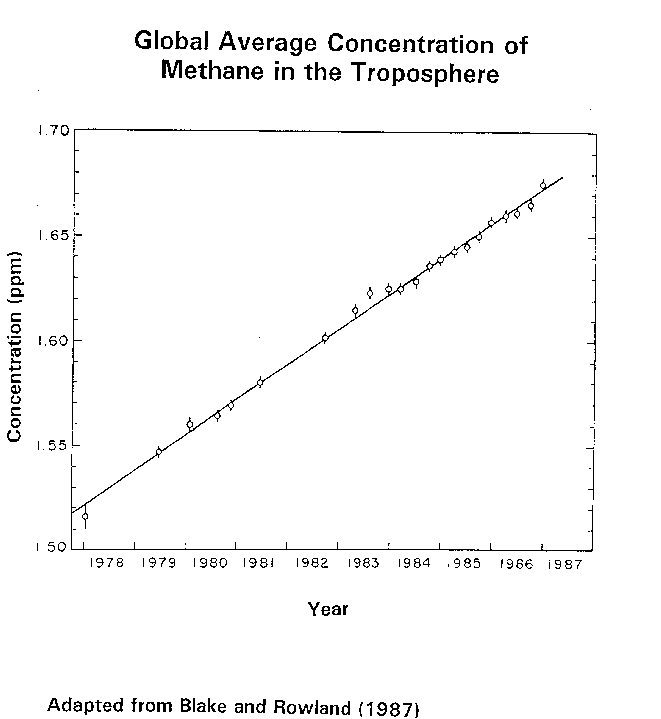
Global concentrations of methane in the troposphere. (Adapted from Blake and Rowland (1987).)
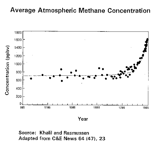Average atmospheric methane concentrations. (Adapted from Khalil and Rasmussen, C and E News, 64 (47), 23.)
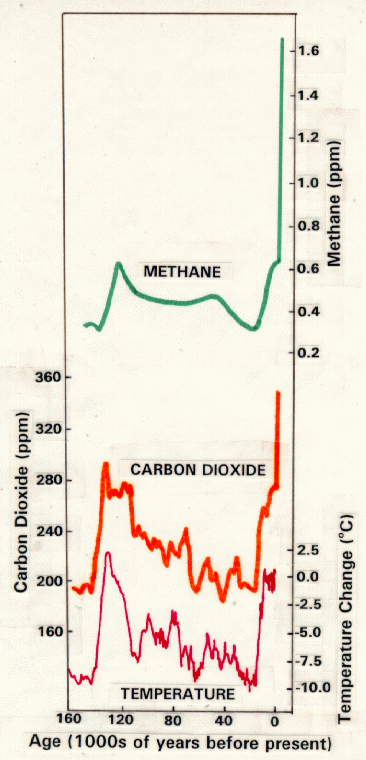Methane, CO₂ and temperature profiles. (Adapted from Woodwell et al, Scientific American, April 1989.)

What are the sources of methane? The 1992 IPCC report lists the largest natural source of methane to be wetlands, which produce 115 teragrams (1012 grams) of carbon annually. The uncertainty in these numbers, however, is very large. Termites are very significant producers of methane in that they eat wood and release methane in the digestion process. The ocean produces about 10 teragrams per year of methane, and fresh water and methane hydrate contribute smaller amounts. 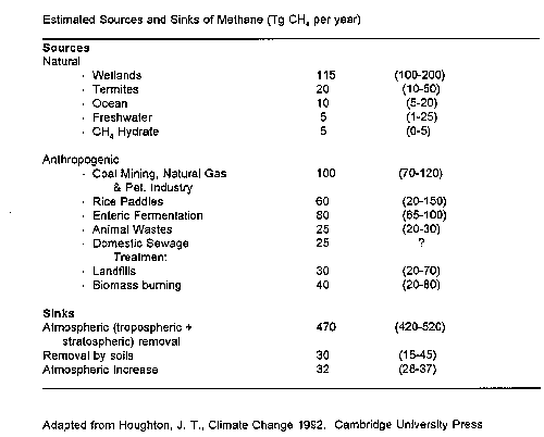Estimated sources and sinks of methane. (Adapted from the IPCC supplemental Report, 1992.)

Anthropogenic sources include coal mining, natural gas and petroleum industry at about 100 teragrams, which is almost as much as natural wetlands. Rice paddies produce on the order of 60 teragrams by means of a process where methane produced in the soil is able to travel up to the hollow stem of the rice plant and be released into the atmosphere without passing through the water which would tend to suppress the evolution of methane gas. 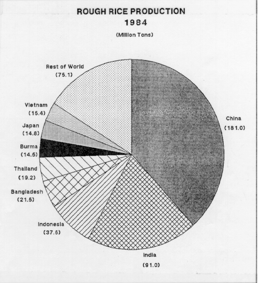As shown in the pie chart from EPA, China is the world's lead producer of rice, followed by India and Indonesia.

Enteric fermentation, the digestion process in ruminant animals such as cattle, sheep and goats, produces very large amounts of methane. Animal wastes produce about 25 teragrams; domestic sewage, 25 teragrams; landfills about 30 teragrams; and biomass burning, about 40 teragrams. Some landfills are now being tapped for their methane as a source of power production. This makes good sense on the basis of global warming in addition to getting a "free" source of combustion gas. Burning one methane molecule produces one CO₂ molecule, but the global warming potential is reduced by a factor of 20 because the carbon dioxide molecule is only about one-twentieth as effective as the methane molecule in absorbing infrared radiation.

Increases in animal populations are contributing to the increase in atmospheric methane. The next plot shows recent increases in several different classes of livestock. If humans continue to have an appetite for meat, the upward trend in animal production and resulting production of methane will likely continue. A particular situation to watch is the development and possible dietary changes in China. If we examine the eating habits of Japan, South Korea, and other Asian nations that have developed very rapidly, one of the significant changes that occurs during economic development is that people's eating habits change from eating primarily grains, mainly rice in these cases, to substantial increases in meat. The big question on the horizon right now is what's going to happen in China? China has an enormous population and it is developing extremely rapidly. If China follows the pattern of other Asian nations, the demand for meat will increase dramatically. I estimated that if you gave every Chinese person 4 Big Macs per year, it would take all of the corn raised in Iowa in a year. 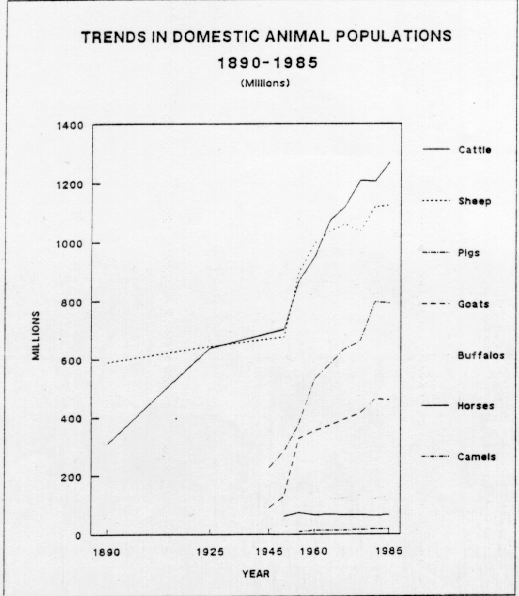Trends in domestic animal population (1890-1985). (From EPA, 1989: Policy Options for Stabilizing Global Climate.)

Sinks for methane include atmospheric removal of about 470 units, removal by soil of about 30 teragrams, leaving an atmospheric increase of about 32 units. By taking subtotals of natural and anthropogenic sources, it is easy to see that humans contribute at least as much as natural sources and possible much more. Such numbers as these are consistent with the observed build-up of methane in the atmosphere in the last 200 years. (See the sources and sinks table above.)

Carbon monoxide is another carbonaceous gas in the earth's atmosphere that participates in the global carbon cycle. The accompanying table gives the sources and sinks of carbon monoxide in teragrams of carbon per year. Fossil fuel combustion is a significant source, as is biomass burning. Carbon monoxide also can be produced in secondary oxidation reactions with methane or non-methane hydrocarbons (NMHC). Major sinks include reaction with the hydroxyl radical and soil uptake. These estimates also carry large uncertainties, but again it is very likely that anthropogenic sources dominate natural sources. Carbon monoxide is much more reactive than carbon dioxide, so its lifetime in the atmosphere is comparably shorter. Measurements of CO and N₂O from satellites are described by NASA. 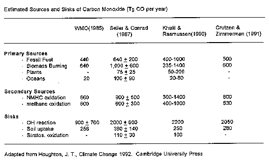Estimated sources and sinks of carbon monoxide. (From EPA, 1989: Policy Options for Stabilizing Global Climate.

Additional summary information.

Transcription by Theresa M. Nichols

Actually, methane is the most rapidly increasing greenhouse gas. The first plot below shows the present concentration of methane, in parts per million by volume (ppm), to be about 1.7 ppm. Sometimes methane concentration is given in parts per billion by volume (ppb), and then would have a value of 1700 ppb. The numerical values show that methane is much less abundant than carbon dioxide which has a present concentration of about 360 ppm. However, the curve shows that the concentration is increasing at about 1% per year. If we look at a longer term, as shown in the second graph below, we see that concentrations have increased substantially since the Industrial Revolution. Estimate of atmospheric methane from a thousand years ago suggest values around 0.7 ppm (700 ppb) which were constant until about the late 1700s. Since that time, concentrations have more than doubled. If we examine the Antarctic ice core data going back 160,000 years, we see that methane levels fluctuated between about 300 parts per billion and 700 parts per billion until the Industrial Revolution when it began its climb to near 1700 parts per billion.
Global concentrations of methane in the troposphere. (Adapted from Blake and Rowland (1987).)	Average atmospheric methane concentrations. (Adapted from Khalil and Rasmussen, C and E News, 64 (47), 23.)	Methane, CO₂ and temperature profiles. (Adapted from Woodwell et al, Scientific American, April 1989.)