1.Introduction

Accurate representation of monthly, seasonal and yearly observations of dew-point temperature is essential to get a complete climatological view of the Upper Midwest. Dew-point temperature is an important tool in forecasting through its use in both the specific and relative humidities. These regulate transpiration and evaporation processes and are key factors in the surface energy and hydrological budgets (Gaffen and Ross, 1999). Because water vapor is the strongest contribution to the greenhouse effect, any changes in dew-point temperatures would have important implications for climate change. The main purpose of this paper is to analyze trends and variability of dew points across the Upper Midwest monthly, seasonally and in a climatological sense.

Dew-point temperature was chosen because it appears to be a more accurate parameter for measuring humidity and has been used more often in studies of climate (Robinson, 1998). Data are also more readily available as most weather stations record dew-point temperatures hourly.

One of the earliest climatological studies on dew-point temperatures was done by Dodd (1965). The study was based upon observations throughout the contiguous United States with approximately 200 stations using psychometric summaries available from 1949-1960. The techniques used by Dodd (1965) will be used in this study to analyze data from the Upper Midwest, as many stations used in this region have data from about 1961 through today.

Seasonal averages show that from 1961 through 1990 there was an increase in dew points through the spring and fall (Gaffen and Ross, 1999). Robinson’s (1998) study showed that there was a change in the dew-point temperature minimum from Minnesota in the winter to the High Plains in the summer, supporting the theory that the Gulf of Mexico is the responsible source of moisture for the east.

Robinson’s study (1998) of the U.S. divided the country into six different “cluster” group areas of similar dew points. The T_d minimum was in January through the entire contiguous U.S., but dew points in the Upper Midwest on average were consistently lower than all other regions through winter.

Over the U.S. during the summer, there was a small positive dew point trend and a more negative pattern in the winter (Robinson, 2000). The same study also showed a diurnal pattern in the summer with rapid increases at midday, suggesting an increase in local evaporation resulting in an increase in humidity.

Peixoto and Oort (1996) show through model simulations of the globe that the atmosphere appears to sustain a fairly consistent distribution of relative humidity over vastly changing temperatures, making an increase in temperature lead to an increase in water vapor along with amplified thermal radiation absorption leading to future increases in temperature.

On a smaller scale there is evidence of a “warming hole” (Pan et al, 2004) in central United States, showing daytime maximum temperatures cooling by 0.2-0.8°C in the summer, due to evaporation of soil moisture that could possibly shrink the effects of greenhouse warming.

An inverse relationship between T_d and inter-annual variability was persistent in Robinson’s (1998) monthly analysis.

Generally across the United States, T_d along with specific humidity have similar spatial and temporal patterns, increasing more overnight than during the daytime (Gaffen and Ross, 1999). Schwartzman et al (1998), however, found that diurnal variations of T_d have little hour-to-hour variation overnight and found a slight increase in the hours following sunset then decreasing towards sunset. In fact it was found that during the warmer seasons the opposite was true and the daytime dew points increased at a greater rate than overnight dew-point temperatures across the United States and Canada.

In a rural setting there is vertical mixing and morning dew evaporates, which raises the dew points at sunrise. In an urban setting, there is less vertical mixing and the dew-point diurnal minimum occurs at or near sunset (Schwartzman et al, 1998).

It cannot be assumed that the records at the stations are completely uniform. As time goes on, technology changes and so do instruments measuring T_d. In the early 1950s, the National Weather Service calculated T_d based on dry and wet bulb temperature observations from sling psychrometers. The dial hygrothermometer was introduced in the 60s. An updated version was later introduced, and the most common sensor used by the NWS is the HO-83. It is also plausible that the instrumental effects could have resulted in a 1.8°F increase in dew points over the 44-year period (Robinson, 2000).

Overall, there was a general increase of 0.9°F per 100 years in dew points over most of the country, with the most dramatic increases occurring over the spring and fall (Robinson, 2000).

In this paper I will examine the hypothesis that dew points have experienced significant, positive trends over the past 44 years in the Upper Midwest. I will also examine the hypothesis that those dew point tendencies are no different from trends that have been found across the rest of the United States.

2.Data and Methods

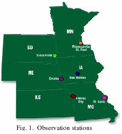
Surface dew point hourly observations were obtained through the Iowa Environmental Mesonet (IEM, 2006) from the National Climate Data Center for six stations throughout the Midwest: Des Moines (DSM), Kansas City (MCI), Minneapolis (MSP), Omaha (OMA), Sioux Falls (FSD), and St. Louis (STL) (Fig. 1). The data were extracted via a Python script that computed monthly averages for each year.

Data were obtained from 1961 to 2005 and were analyzed to find the monthly, seasonal, yearly and decade trends. (Data were only available in Kansas City and St. Louis from 1973 to 2005 and in Omaha from 1974 to 2005)

The seasons defined in this analysis will be consistent with Schwartzman et al (1998) with winter months of December, January, and February; spring consisting of the months of March, April and May; June, July and August composing the summer season; and fall comprised of September, October and November.

When individual hourly data were missing, they were left out of the analysis and averages were based upon the available data. From 1961-2005, the percent of missing data for each station was: Sioux Falls, 0%; Minneapolis, 18%, due to a data gap; Omaha, 30.11% as a result of no data before 1974; Des Moines, 1.33% due a data gap; Kansas City, 27.27% a result of no data before 1973; and St. Louis, 27.27% as a result of no data before 1973. To account for the missing data gap in Minneapolis, the decadal average was filled into the missing years and the trend was not significantly affected so the data was not used. Nearest neighbor data filling could be used to ameliorate the missing data in future studies.

Days with dew points over 70, 75 and 80 °F were analyzed separately by month, season, year and decade also.

Trends were tested for significance based upon the linear p-value. This was calculated using the statistics program: JMP (Statistical Discovery, 2005) and output the observed significance probability calculated from each t-ratio (tests the hypothesis that each parameter is zero, ratio of the parameter estimate to its standard error). The value is the probability of getting, by chance alone, a t-ratio greater than the computed value, given a true hypothesis. Data in this thesis were considered significant if the p-value was below 0.05, making the trend significantly different from zero.

3.Results

3.1. Monthly climatic trends

Data from 1961 to 2005 revealed several trends in monthly mean dew-point temperatures. (Table 1) The most significant trends occurred in January, February, July, August and December in nearly all of the stations.

The largest trends in dew point throughout the 44-year period occurred in January. This is also the month where these positive slopes had the highest significance for all stations. Averaged over all stations, dew points were increasing by 0.22°F per year during the period. There was no spatial trend evident in January.

February also had a statistically significant positive linear correlation in Kansas City, Sioux Falls, Minneapolis and Des Moines. Dew points were increasing by 0.14°F per year on average during this month.

In December, there was also an increase in dew points over the specified period. The dew point boost was prevalent mainly in the north, where the increase was most significant in Minneapolis and Sioux Falls. Smaller increases occurred in the south, with the smallest increase being in St. Louis.

During the summer, August had the most statistically significant positive slope, averaged to be 0.084°F per year over the six stations used. Sioux Falls, Kansas City, Des Moines and Omaha all had p-values less than 0.05. There was no correlation between location and magnitude of the increased dew points during August.

July was the final month that showed significant positive increases in dew point throughout the period. There was an overall increase averaged in the six cities of 0.070°F per year with no correlation to the position of the observation stations. July was the final month that showed significant positive increases in dew point throughout the period. There was an overall increase averaged for the six cities of 0.070°F per year with no correlation to the position of the observation stations.

FSD	Jan	Feb	Mar	Apr	May	June	July	Aug	Sept	Oct	Nov	Dec
Slope	0.27	0.15	0.052	0.055	0.061	0.037	0.086	0.13	0.075	0.0037	0.027	0.14
P-Value	0.0008	0.027	0.23	0.089	0.19	0.31	0.0032	0.0001	0.024	0.94	0.55	0.032
MPLS	Jan	Feb	Mar	Apr	May	June	July	Aug	Sept	Oct	Nov	Dec
Slope	0.083	0.15	0.035	0.044	0.0088	0.03	0.042	0.06	0.051	-0.016	0.011	0.2
P-Value	0.0068	0.093	0.55	0.28	0.87	0.4	0.17	0.079	0.23	0.76	0.85	0.02
OMA	Jan	Feb	Mar	Apr	May	June	July	Aug	Sept	Oct	Nov	Dec
Slope	0.26	0.15	0.039	0.0019	0.04	0.073	0.086	0.088	0.025	0.09	0.071	0.12
P-Value	0.016	0.19	0.61	0.98	0.6	0.15	0.05	0.053	0.67	0.17	0.4	0.27
DSM	Jan	Feb	Mar	Apr	May	June	July	Aug	Sept	Oct	Nov	Dec
Slope	0.22	0.14	0.07	0.053	0.048	0.035	0.07	0.09	0.014	0.024	0.021	0.094
P-Value	0.0025	0.035	0.13	0.12	0.34	0.28	0.0043	0.0021	0.69	0.59	0.67	0.17
MCI	Jan	Feb	Mar	Apr	May	June	July	Aug	Sept	Oct	Nov	Dec
Slope	0.31	0.18	-0.022	0.089	0.092	0.083	0.12	0.11	0.042	0.092	0.092	0.14
P-Value	0.0012	0.076	0.76	0.19	0.2	0.073	0.019	0.0087	0.46	0.19	0.27	0.18
STL	Jan	Feb	Mar	Apr	May	June	July	Aug	Sept	Oct	Nov	Dec
Slope	0.19	0.087	-0.11	0.059	0.041	0.023	0.014	0.033	-0.035	0.037	-0.031	0.0084
P-Value	0.036	0.33	0.11	0.3	0.6	0.63	0.72	0.46	0.5	0.58	0.69	0.93

Table 2. Monthly trends of dew-point temperature and P-values (where P-value <0.05 and P-value <0.1)

3.2. Seasonal climatic trends

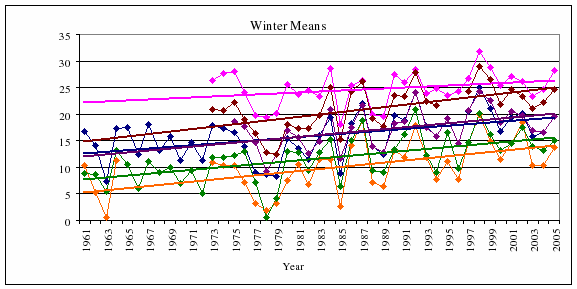
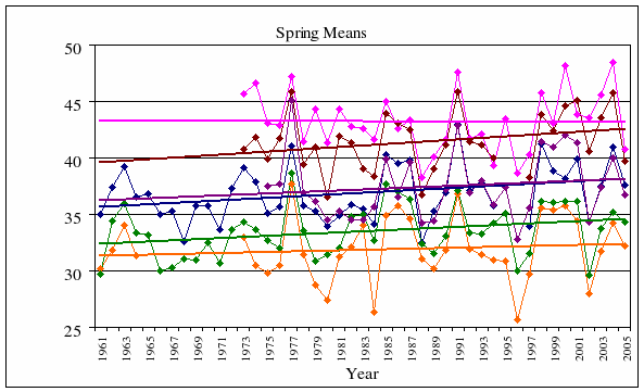
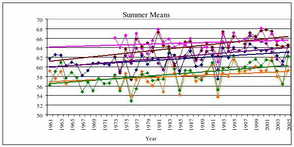
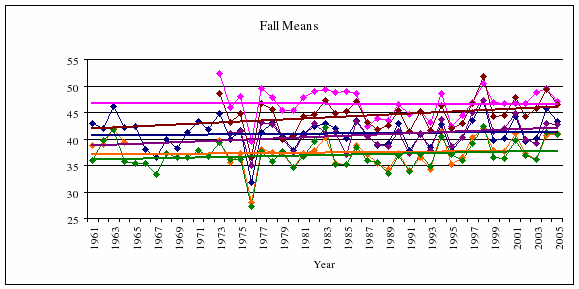
Each season had a positive dew point trend through the 44-year period. This agrees with Gaffen and Ross (1999) but the greatest and most significant increases were found to be in the winter and summer months in this study as opposed to in the spring and fall in this study where the increases were not as steep or significant (Fig. A2 and Fig. A3). This discrepancy could be due to the fact that the Gaffen and Ross study was over the entire nation versus one section of the nation.

Table 1. Monthly trends of dew-point temperature and P-values (where P-value < 0.05 and P-value < 0.1)

Results of this study nearly match Robinson’s (2000) findings during the summer months (Fig. A3), where the most significant positive trend was during the summer months throughout the United States. Observations showed the summer months (June, July and August) to have had the second main rise in dew-point temperatures. The mean increase in the region was 0.070°F per year with Kansas City, Sioux Falls, Omaha and Des Moines all having significant positive tendencies during this time.

3.3. Yearly average climatic trends

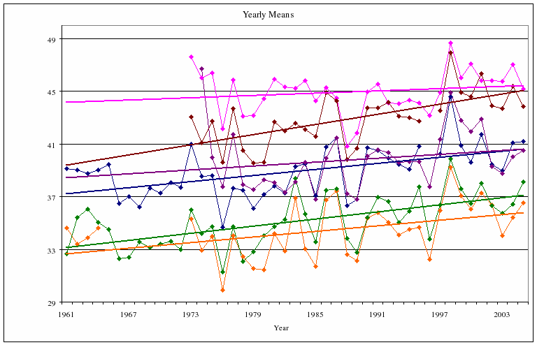
This study showed agreement with a general increase in dew-point temperatures through time, but the increase is quite different comparatively. Averaging the slopes of the observation stations yields an area increase of approximately 7.54°F per 100 years (Fig. A5) compared to the 0.9°F per 100 years found by Robinson (2000). This suggests that the region in this study could be partly responsible for the nationwide increase.

3.4. Decadal climatic trends

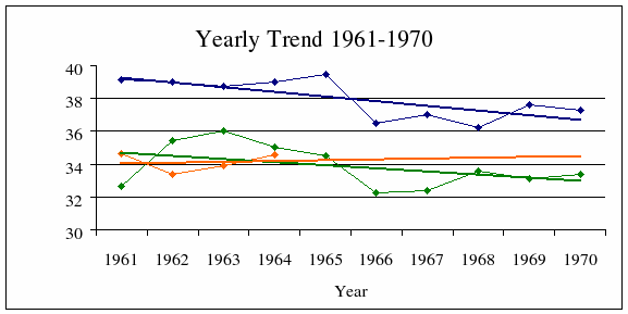
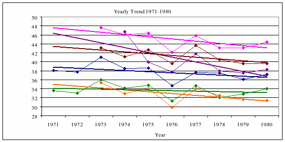
Although most of the trends through the decades generally did not show significant trends, it can be seen in Fig. A6 and Fig. A7 that there is an overall negative pattern in the yearly means between 1961 and 1980.

From 1961 to 1970, Des Moines has a significant negative trend. But when the dew points are considered throughout the duration of the study, there is a significant positive trend. St. Louis also has a slightly significant negative trend from 1971 to 1980 and then again from 1981 to 1990. But between 1991 and 2000, the trend switches to being a positive slightly significant pattern, which shows quite an apparent switch in the trend.

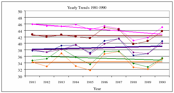
Averaging the six observation stations between 1981 and 1990 (Fig. A8), there is a relatively neutral slope, leaning slightly negative. This is due to St. Louis, Sioux Falls, and Kansas City all exhibiting a more negative pattern while Minneapolis, Des Moines and Omaha all showing a slightly positive trend.

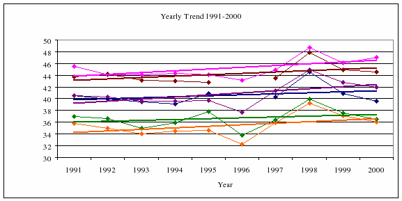
All cities show a positive correlation from 1991 onward (Fig. A9). Since the yearly average trends all exhibit significant increasing patterns, the reversal in dew-point trends occurred sometime in the past 20 years and has made a large impact on the average trends over the past 44 years.

3.5. Twenty-two-year trends

By dividing the time period in half, trends were more apparent.

From 1961 until 1983 each observation station, except Sioux Falls showed a negative trend. This pattern was significant in Omaha where the slope was the steepest.

From 1984 until 2005, every city had an increase in dew points, with significant trends in Des Moines and St. Louis and slightly significant trends in Minneapolis and Omaha.

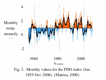
Again, there is a switch from a negative to a positive trend occurring somewhere in the late seventies. This switch may be related to the Pacific Decadal Oscillation (PDO). There is argument that the trends since the seventies are occurring as a result of a superposition of a wet phase of the PDO in addition to the global increasing trend. A “cool” PDO regime was apparent from 1947-1976, where it then switches between 1976 and 1977 to a more “warm regime” as seen in Fig. 2 (Mantua, 2000).

3.6. Extreme days

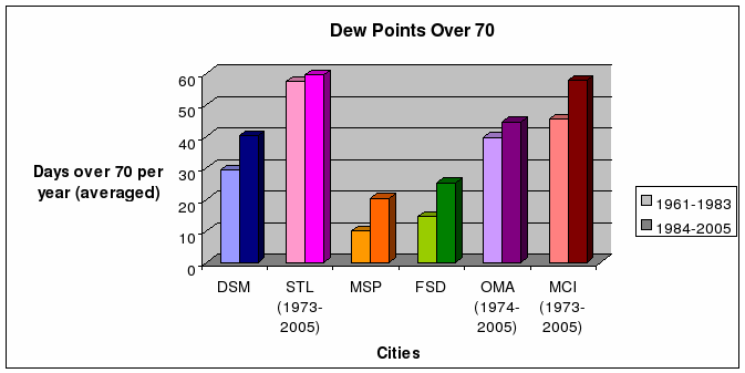
Extreme days where the dew points were over 70°F and over 75°F were analyzed using the twenty-two year periods. At each station, the number of days with dew points over 70°F in the second period (1984-2005) was higher than the number of days in the years preceding (Fig. A10).

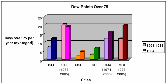
Similar results were found in days over 75°F with most stations having up to twice as many extreme cases in the later period (Fig. A11).

This shows that not only are dew points in general increasing, but days with extremely high dew points are becoming more numerous also. It is noteworthy that the number of days with extreme dew points showed closer correlation between the two periods in St. Louis, Omaha and Kansas City, where data was only available from 1974, which could show that the number of extreme dates was higher at the end of the first period.

3.7. Precipitable Water

Based on the increase in dew points, the precipitable water over an area can be found. It gives an idea of how much more water is input into the atmosphere. In this study the precipitable water was found purely based upon the dew point temperature. As Butler (1998) derived the surface water vapor pressure as P_o to be as stated in Equation 1, with D being the dew-point temperature.

Equation 1. Surface vapor pressure (mb).

P_o = 1mb*e ^{{1.81+(17.27*D)/(D+237.3)}}

Assuming an isothermal atmosphere in hydrostatic equilibrium the precipitable water (h) would be as stated in Equation 2.

h = P_o /(ρ_w*g)

Where ρ_w is the density of water, taken to be 1000 kg/m³. And g is the mean gravitational acceleration of the Earth, approximately 9.81m/s².

The mean dew-point temperature at the first year and the last year of the observation period was put into this formula, and the difference in precipitable water was found and extrapolated over the duration of 100 years to determine if the increase in precipitable water would be significant.

Data were analyzed for the yearly observations and for the winter and summer months (Table 2).

Table 2. Precipitable water amounts (mm/100 years)

This yields an average of 0.27 millimeters of precipitable water over 100 years. Precipitable water amounts in the winter months were over double the summer amount of precipitable water in Des Moines and Minneapolis. While the summer months in Omaha and Kansas City were nearly double the winter months in precipitable water amounts.

4.Implications

Equation 2. Precipitable water (m).

With the increase in dew-point temperature, agricultural animals and production processes may also be influenced. All animals have a thermal neutral zone where their performance is optimal and once outside of this zone, their performance decreases. This zone may be becoming smaller with the increase in dew points and decrease in daytime maximum temperatures.

One of the first impacts of heat stress on market animals such as hogs and cattle is a drop in food consumption (Stalder, 2006). The largest economic issue with animal heat stress is the reduction of productivity, whether putting on weight for meat production or poultry. The second issue is increased mortality rates; this is prevalent in the summer months where agricultural animal fatalities spike (St-Pierre et al, 2003). The third economic issue is the decline in the product quality (Stalder, 2006).

Such a large overall increase in dew points and potentially precipitation through the years, if it continues, will affect crop production, soil erosion, water supplies and human health. For instance, trends found a higher occurrence of dew-point temperatures exceeding 75°F; this is likely to intensify the impacts of heat waves in major cities.

5.Concluding Remarks

Based upon the data in this study it is evident that there is a positive trend in dew point over a 44-year period, particularly in the past twenty years. In the beginning of this period in the Upper Midwest, there is a decrease of dew points in all cities in this region. But there is an apparent shift to a significant positive slope in dew points over the months, seasons, decades and duration of the study.

The recent changes in trends in dew-point temperatures exposed in this study have important implications for regional agriculture, water supplies and human health. Modeling studies should be carried out to try to pin down the underlying courses for their changes. This may clarify whether increases in greenhouse gases, the PDO, El Niño, Atlantic Oscillation or some other factor is responsible for these trends.

The hypothesis that dew points have experienced significant, positive trends over the past 44 years in the Upper Midwest holds true in this study. The research presented shows an overall positive trend in dew-point temperature through the Upper Midwest during the past 44 years. The hypothesis that the dew-point temperature tendencies are no different from trends that have been found across the rest of the United States is false however. The Upper Midwest region shows a more significant positive trend when compared with the United States as a whole with the Upper Midwest dew-point temperatures increasing by 7.54°F over 100 years, compared to the 0.9°F over 100 years in the U.S.

6.Acknowledgements

Thanks to Daryl Herzmann for writing the Python script to retrieve the data from the National Climate Data Center, for his guidance and constructive suggestions. Thanks also to Dr. Eugene Takle and Jon Hobbs for their assistance and comments.

7.References

Butler, Bryan, 1998: Precipitable Water at the VLA --1990-1998. MMA Memo. No. 237, 8 pp.

Dodd, A.V., 1965a: Dew point distribution in the contiguous United States. Mon. Wea. Rev., 93, 113-122.

Gaffen, D.J., and R.J. Ross, 1999: Climatology and trends of the U.S. surface humidity and temperature. J. Climate, 12, 811-828.

Pan, Z., R.W. Arritt, E.S. Takle, W.J. Gutowski Jr., C.J. Anderson, and M. Segal, 2004: Altered hydrologic feedback in a warming climate introduces a “warming hole". Geophys. Res. Lett., 31, L1709.

Peixoto, J.P. and A.H. Oort, 1996: Climatology of relative humidity in the atmosphere. Int. J. Climate, 9, 3443-3463.

Robinson, P.J., 1998: Monthly variations of dew point temperature in the coterminous United States. Int. J. Climate, 18, 1539-1556.

Robinson, P.J., 2000: Temporal trends in United States dew point temperatures. Int. J. Climate, 20, 985-1002.

Ross, R.J., and W.P. Elliot, 1996: Tropospheric water vapor climatology and trends over North America: 1973-93. J. Climate, 9, 3561-3574.

Schwartzman, P.D., P.J. Michaels, and P.C. Knappenberger, 1998:Observed changes in the diurnal dewpoint cycles across North America. Geophys. Res. Lett., 25, 2265-2268.

Stalder, Ken, 28 November, 2006. Personal communication.

Statistical Discovery, 2005: JMP- Version 6.0. SAS Institute, Inc.

St-Pierre, N.R., B. Cobanov, and G.Schnitkey, 2003: Econmonic Losses from Heat Stress by US Livestock Industries. J. of Dairy Science, 86, E52-E77.