Meteorology 454 - Wave Analysis Project

Fall 2019

1. How rapidly to wave patterns move?

2. How long does one identifiable pattern last?

3. How rapidly to waves increase or decrease in amplitude?

4. How does zonal wind evolve through the period?

5. Is there a relationship between zonal wind speed and wave propagation?

6. Is there a relationship between zonal wind speed and wave growth/decay?

Students will be assigned observing teams. Teams will access animations of 500 hPa heights and zonal jets to observe and record behavior until shortly before Thanksgiving. The assembled database will be a record of wave evolution in the atmosphere. Teams will perform analyses described below to diagnose behavior of large-scale, synoptic waves and compare it with Rossby wave theory. Analyses will be reported shortly after observations stop.

The animations are located at the Iowa State Weather Products page. This site contains continually updated, (near) real-time weather products. This project focuses on the Upper Air Analysis: Hemispheric Plots, specifically

• Northern Hemisphere 500 hPa heights
• Southern Hemisphere 500 hPa heights
• Global zonal average zonal wind

Let's look at each one in turn:

Select the "Northern Hemispheric 500MB" link, ignoring the "(8 day loop)" for the moment. A color contour plot will appear showing the most recent 500 hPa height field for the Northern Hemisphere. Height contours are every 60 meters. The heights appear as a wave-like field encircling the North Pole. Thick white lines overlying the contours outline the continents, thin lines show latitude every 10 degrees from the pole and longitude every 10 degrees east-west. (The 100 degrees west line runs through Texas and North Dakota.) Below the figure is the date/time stamp.

Click the "Back" button, then select "(8 day loop)" adjacent to the Northern Hemisphere 500 hPa link. You will need to be patient while the loop loads. It gives an 8-day sequence of 500 hPa color contour plots, animated for viewing. Which way do the wave patterns move?

Note the buttons on the left side. These can control speed of animation and also allow you to step through the sequence one plot at a time. Try using the buttons to understand how they work, as they will be useful for this project.

These show the same fields as (a), but for the Southern Hemisphere. Where is Antarctica? Which way do the waves move here? Why?

The third link, "Global Zonal Wind Average", shows the east-west wind averaged in longitude, the so-called "zonal average". It is plotted as a latitude-height cross section, which allows us to view both hemispheres at once. The South Polar region is on the left, the North Polar Region is on the right. Why do you think there are blank places (colored white) along the bottom?

Considering the GOALS and QUESTIONS TO CONSIDER for this project, there are several features of the wavelike behavior that should be recorded: motion, amplitude, dominant wavelength.

We also need to consider the environment in which the wave is embedded, which is why the zonal wind cross-section is given. Items to observed and record would be maximum speed in each hemisphere and latitude of the maximum speed, near the latitudes where the waves occur. It will be useful (potentially) to know the wind at a couple of levels, so I recommend recording, at roughly 50 deg latitude for each hemisphere, the zonal wind speed at 500 hPa and in the layer 150 - 300 hPa.

Data should be recorded for each day.

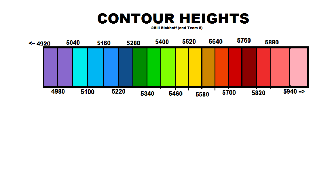
An important question here is: what part of the wave should we measure? One simple way is to focus on a single contour. Look at the Northern Hemisphere, a pick out a contour that is somewhere in the middle of the range of heights and that exhibits a moderately clear west-east movement. Consider the figure below. I suggest the 5580 m contour, which separates yellow and orange color zones.

For the Southern Hemisphere, I suggest the 5280 contour, which separates blue and green color zones.

(b) Wavelength (wavenumber)

Estimating the dominant wavelength can be rather tricky, as the height field is likely composed of several waves. I suggest a fairly simple counting method, focusing on one latitude circle, 50 degrees north. The latitude circle 50 N passes just north of the Canada-U.S. border, through northern Europe, through the Mongolia-Siberia border and just south of the Aleutian Islands. Simply start at some longitude and count the number of times the 5580 m contour crosses 50 N. Do not count times when the contour lies on but does not cross 50 N. You should end up with an even number. The estimated integral wave number N is one half of the crossings. In the example above, there are 6 complete crossing of 50 deg latitude, so N = 3.

For the Southern Hemisphere, I suggest using 50 degrees south. In the example above, counting crossings of 50 S by the 5280 m contour gives N = 3.

Again, N should be recorded for each day for each hemisphere.

Strictly speaking, amplitude A should be estimated from

A = (Zmax - Zmin)/2

where Zmax is the maximum height for wave number N as one goes around a selected latitude circle, and Zmin is the minimum height. However, determining Zmax and Zmin can be difficult because there are likely several waves present in addition to our estimated dominant wave. Going around the 50 deg. latitude circle, we encounter a local maximum in height between successive pairs of 5580 m crossings toward higher and then lower heights. This means we have N local height maxima going around the latitude circle. Similarly, we have N local height minima. I suggest estimating the amplitude by taking

AveMaxima = average of the N local height maxima
AveMinima = average of the N local height mimima

A = (AveMaxima - AveMinima)/2

The animation loop will be especially helpful here. We need to mark the movement of a wave. I suggest choosing one point where the target contour crosses the target latitude circle and following its movement from day-to-day. Record the longitude of the feature on each day. Then compute the speed C for a given day as

C = {LON(day+1) - LON(day-1)} /2

That is, speed is estimated as one half the change in longitude between the day after and the day before.

It would be even better to do this for more than one crossing point to get a more representative value.

(e) Zonal wind