2-6: Soil-Vegetation-Atmosphere Modeling

Eugene S. Takle
© 2000, 2002, 2004, 2006

Much of this information has been taken from:

Sellers, P. J., and Y. Mintz, Y. C. Sud, A. Dalcher, 1986: A simple biosphere model (SiB)
for use within general circulation models. Journal of the Atmospheric Sciences, 43, 505-531.

Introduction

The surface of the earth is the gateway for energy (heat), moisture, and trace gases to enter or leave the atmosphere. It also is where kinetic energy of mass motion is extracted from the atmosphere. Global and regional climate models require accurate information on the rates of input of heat and moisture and extraction of momentum (kinetic energy). An amount per unit time of some quantity (heat, mass, momentum, etc) passing through a surface is known as a flux. Soil-vegetation-atmosphere transfer models (SVATs) are used to link to global and regional climate models to more accurately describe how soil, vegetation, and water surfaces exchange fluxes with the atmosphere.

Development of SVAT Models

Plants interact with the atmosphere in a variety of ways, but only recently have scientists been able to describe these interactions mathematically through the use of SVAT models.

Development of SVAT models has come from the convergence of two needs:

• Meteorologists and climatologists need information on the heat and moisture input to the atmosphere from the earth's surface (e.g., soil, vegetation, water bodies) and how the surface extracts momentum and kinetic energy of the atmosphere through "friction".
• Biophysicists and ecologists need information about the temperature, humidity levels, solar radiation, cloud cover, wind speed, precipitation, etc. to determine how plants and plant communities respond to environmental conditions. Neither of these scientific communities had sufficient computing power to consider how the vegetation and atmosphere interact and feedback to each other. For instance, a long run of days with hot, dry conditions will force plants to use up all available soil moisture, after which they will wilt (quit transpiring water) and turn brown or more silver green. Their plant behavior changes the atmosphere ( in a small but perhaps significant way) by reducing a moisture source and having more solar energy reflected by the wilting plants.

Prior attempts to link these two groups took the form of meteorologists using fixed vegetation conditions and plant physiologists using fixed climate conditions.

SiB Model

The SiB model provides a link between these two groups that allows plants to interact with changing atmospheric conditions, and these atmospheric conditions are determined, in part, by the role of vegetation in governing evaporation, absorption of solar radiation, interception of precipitation, etc. SiB allows for two-way interactions between the atmosphere and the biosphere/lithosphere.

1. Radiation absorption
   Plants in SiB absorb energy very effectively in the wavelength interval 0.4 to 0.72 microns (the photosynthetically active radiation, or PAR, portion of the solar spectrum).
   Plants in SiB reflect radiation in the near infrared portion of the spectrum.
   Bare ground in SiB has a gradual increase in reflection with wavelength from 0.4 to 4.0 microns.
2. Biophysical control of evapotranspiration
   Stomates ( timy openings in plant leaves) control the interchange of water and CO₂ between the atmosphere and the plant.
   Vegetation canopies intercept and hold precipitation and dew, which lowers water input to the soil and enhances evaporation.
3. Momentum transfer
   Plants create "friction" for the atmospheric flow near the surface. Plants create turbulent motions that enhance vertical mixing of heat and water vapor near the surface.
4. Soil moisture availability
   Plants in SiB have roots that determine the amount of water available for evapotranspiration.
5. Insulation
   SiB has live plants that shade the surface and protect it from intense solar radiation and strong evaporation.

Atmospheric Properties Changed by SiB

Here we describe the terms from the atmospheric model that are changed by SiB and the properties of the plants and surface that change and influence the atmospheric conditions.

a) Atmospheric variables given to SiB

1. Temperature, vapor pressure, and wind speed.
   * variables represent grid-averaged values
   * temperature, T_r
   * water-vapor pressure, e_r
   * wind speed u_r
2. Radiation
   * Visible or PAR (< 0.72 microns, direct beam) F_s,b(0)
   * Visible or PAR (, 0.72 microns, diffuse) F_s,d(0)
   * Near infrared (0.72 - 4.0 microns, direct beam) ) F_n,b(0)
   * Near infrared (0.72 - 4.0 microns, diffuse) F_n,d(0)
   * Thermal infrared (> 4.0 microns, diffuse) F_t,d(0)
   F_s is absorbed for photosynthesis by the leaves, and F_n is primarily scattered. Some light arrives at the leaves, not directly from the solar beam but reflected (sometimes with multiple reflections) off other leaves or higher levels of the canopy.
3. Precipitation
   GCMs or regional climate models calculate precipitation accumulated at the surface over the time step of the model ( a few minutes to a few hours).

b) Components of Sib that change atmospheric properties

1. Two types of vegetation;
   * Trees and shrubs
   * Ground cover

Roots are different for each type of vegetation
2. Rooting zones:
   * Layer 1: upper thin layer which allows direct soil evaporation
   * Layer 2: has roots of annual plants that may grow down to the bottom of this layer with time; has tree and shrub roots at the bottom of this layer
   * Layer 3: this layer collects water that percolates slowly through to the ground water reservoir.

The different types of land surface that are considered in SiB are depicted in Figure 1a. Later versions of SiB have reduced the number of such categories, but other similar models have similar categories. The three-layer soil zone used by SiB2 is shown in Figure 1b.

Representing Plant Functions in Sib

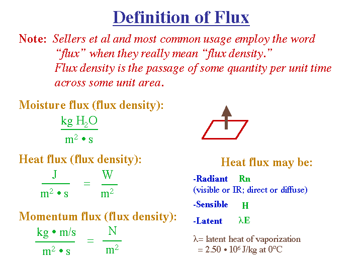
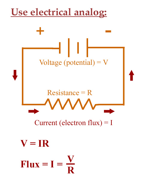
SVATs are constructed to give proper representation of the flow of mass, momentum, energy, and trace gases (e.g., water vapor, CO₂) between the surface and the atmosphere. The flow of these quantities in a unit of time is called flux. The definitions of heat, mass, and momentum fluxes are given in Figure 3. The fluxes are related to measurable variables (like temperature or relative humidity) by use of a simple electrical resistance analog (Figure 4c): V = I x R, where V is voltage (sometimes called the potential difference), I is electrical current, and R is resistance. The flux is analogous to the current, I = V/R. Figure 4d gives the method for calculating, say, the heat flux out of the plant canopy in terms of the potential difference (essentially the difference between the temperatures of the air and canopy) and the "resistance" of the atmosphere. Similar expressions are given for other heat fluxes and also the fluxes of water vapor from the plants and the soil surface.

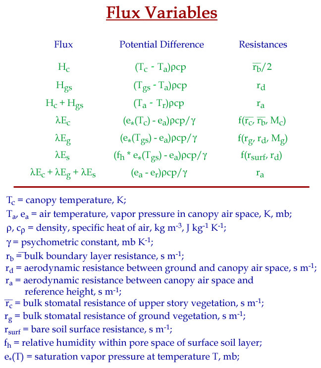
A schematic depicting the various resistances for the atmosphere, plant canopy, ground cover plants, and soil is given in Figure 5. A detailed depiction of the plant stomates in Figure 6 shows that when the stomates open to allow carbon dioxide to flow in, they also allow water vapor to flow out. The plant thereby uses the size of the stomatal opening to regulate its uptake of CO₂ and also to keep it cool by allowing water to evaporate within the stomate and escape to the atmosphere.<

From these definitions, as shown in Figure 7 , we can develop equations for the conservation of energy (equations 1 and 2) and conservation of water substance (equations 3 and 4). In a similar way, equations describing soil wetness in each of the three soil layers can be assembled from the conservation of water as shown by equations 5, 6, and 7 of Figure 8.

The various classes of vegetation are given in Table 2 of Figure 9. When a SVAT is used in conjunction with a global or regional climate model, each grid cell of the climate model must have a "land-use" class given in Table 2 of Figure 9.

A plant physiologist likely would consider these representatives of plant processes to be quite simplistic. However, experiments have shown that global and regional models that represent surface processes by SVATs such as SiB give more accurate simulation of basic climate variables.