 Atmospheric
concentration of from a) 1977-1988 and b) the last 200 years. Houghton, J.T., G.J. Jenkins, J.J. Ephraums, eds,
1990: 1990 Intergovernment Panel on Climate Change, Cambridge
University Press.
Atmospheric
concentration of from a) 1977-1988 and b) the last 200 years. Houghton, J.T., G.J. Jenkins, J.J. Ephraums, eds,
1990: 1990 Intergovernment Panel on Climate Change, Cambridge
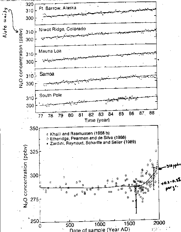
University Press. In this lecture we examine another trace gas in the atmosphere whose concentrations are observed to be increasing. Nitrous oxide, , is a colorless, odorless, non-reactive gas that is very stable in the troposphere (lifetime of 110-168 years). It should not be confused with , NO, or other oxides of nitrogen. Nitrous oxide concentrations have been steadily increasing with time, as shown on the accompanying plot which reports measurements at several locations since 1977. It is important to note that the units of these measurements are part per billion by volume (ppbv). Nitrous oxide concentrations then are about one fifth of methane concentrations and about a thousand times smaller than carbon dioxide.
Atmospheric
concentration of from a) 1977-1988 and b) the last 200 years. Houghton, J.T., G.J. Jenkins, J.J. Ephraums, eds,
1990: 1990 Intergovernment Panel on Climate Change, Cambridge
University Press.
Data over a longer time scale as derived from ice cores show that over the last 2,000 years nitrous oxide concentrations were nearly constant at about 280 ppbv until about the beginning of the Industrial Revolution, at which time there began a fairly dramatic increase which continues today at about 0.2 to 0.3% per year.
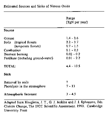 Estimated sources and sinks of nitrous oxide. Adapted from table
1.4, p 26, of Houghton, J.T., G.J. Jenkins, J.J. Ephraums, eds, 1990:
1990 Intergovernment Panel on Climate Change, Cambridge University
Press.
Estimated sources and sinks of nitrous oxide. Adapted from table
1.4, p 26, of Houghton, J.T., G.J. Jenkins, J.J. Ephraums, eds, 1990:
1990 Intergovernment Panel on Climate Change, Cambridge University
Press.
We know the sources of nitrous oxide. Natural sources include oceans, tropical soils, wet forests, dry savannas, and extra-tropical forests. Total emissions are about 4-10 x 1012 grams, or 4-10 Tg. Anthropogenic sources include cultivated soils (including use of nitrogen fertilizers), biomass burning and other combustion processes, and acid production processes. The largest known process for destruction of nitrous oxide is stratospheric photolysis (breakdown by solar energy, principally ultraviolet radiation). From these estimates we can see that in spite of large uncertainty, human contributions to the nitrous oxide loading of the atmosphere are comparable with natural sources and are likely the cause of the 3-4.5 Tg per year increase in the amount of nitrous oxide in the atmosphere. Because of their long lifetime (stability) in the troposphere, natural removal processes are incapable stemming this increase.
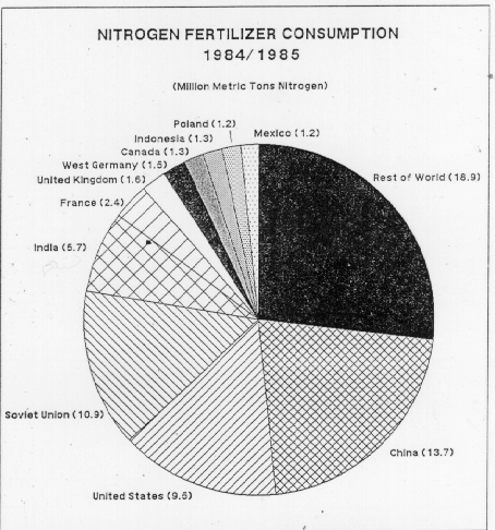 Nitrogen
fertilizer consumption. EPA.
Nitrogen
fertilizer consumption. EPA.
Agricultural use of nitrogen fertilizer is a significant anthropogenic source of nitrous oxide. As shown on the pie chart, China is a big user, followed (according to these data) by the former Soviet Union, the United States, and India. During talks with state officials on my recent trip to Russia, I learned that the present economic difficulties in that country have significantly reduced their availability of fertilizers and pesticides, so this chart may not reflect current conditions.
In a later learning unit we will be coming back to the physics and chemistry of the stratosphere and will revisit the problems caused by nitrous oxide in the stratosphere.
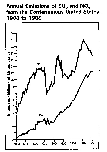 Annual emissions of
and
from 1900-1980. EPA.
Annual emissions of
and
from 1900-1980. EPA.
Other oxides of nitrogen also are being added to the atmosphere in increased amounts. Anthropogenic emissions of nitrogen compounds in the US, as reported by EPA, are shown in the next plot.
 Estimated sources of Nitrogen Oxides.
Adapted from IPCC, 1992. EPA.
Estimated sources of Nitrogen Oxides.
Adapted from IPCC, 1992. EPA.
NO and are gases are collectively taken together with aerosol to comprise what we call . Annual emissions in the US over the last 80 years have increased dramatically, from less than 1 to about 22 Tg (teragrams, or millions of metric tons). On a global basis natural sources of include soils (5-20 Tg annually) and lightning (2-20 Tg annually) and give an annual total amount of 8 to 41 Tg. Anthropogenic sources contribute annually about 27 to 38 Tg from fossil fuel combustion, biomass burning, and tropospheric aircraft. These number suggest that humans are emitting oxides of nitrogen to the atmosphere in total annual amounts that are comparable in magnitude to natural sources.
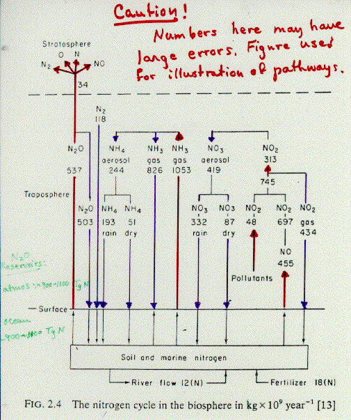 Nitrogen cycle.
J. D. Butler, Air Pollution Chemistry, 1979
Nitrogen cycle.
J. D. Butler, Air Pollution Chemistry, 1979
In order to understand how nitrogen moves throughout the earth/ocean/atmosphere environment, we need to look at the nitrogen cycle, which gives the sources and sinks of nitrogen and the fluxes between these reservoirs, as shown in the above figure. These values may be subject to large errors and are for illustration only. The main concept to draw from this figure is that there are two components of the nitrogen cycle: the right hand side represents tropospheric interactions and interchange with the surface for , and the left hand side describes nitrous oxide, which is considered separately. The components on the right hand side are all part of the rapid cycle: being quite reactive, these constituents will cycle into and out of the lower atmosphere within a couple weeks. But, of course, since we continue to put in more all the time, there is this continuous supply in the atmosphere. However, if we were able to switch off all of natural and anthropogenic sources, the atmospheric concentrations would rapidly deplete to zero within a couple of weeks.
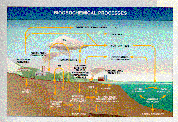 Biogeochemical Processes. U.S. Global Change Research Program.
Also shown are the different pathways and transformations throughout these various cycles. So, for instance, some nitrogen enters the atmosphere as NO, is transformed to , and then may go back into the soils as or it may be converted to in an aerosol and then either rained out or deposited out as a dry particle. The gas may form into particles directly or attach to rain droplets and eventually end up back in the soil or in the ocean. A similar description applies to the various transformations of ammonia ().
Nitrous oxide, on the other hand, follows a different pathway: it experiences no chemical transformation or rainout or dry deposition in the troposphere. Once emitted, the nitrous oxide molecule drifts throughout the lower atmosphere, possible for decades, until it makes a chance visit to the lower stratosphere where it is broken down by ultraviolet light into O and N or NO. The Ns can form , but the NO is available to participate in ozone depletion. The point of this diagram is that, of the nitrogen compounds emitted at the surface by natural or anthropogenic process, only nitrous oxide lives long enough to migrate to the stratosphere to create problems at that level. Oxides of nitrogen in the lower atmosphere cause acid rain problems, as we will see later, but they do not contribute significantly to global warming or ozone depletion.
There are several unanswered questions relating to nitrogen movement through the biosphere, atmosphere and soil. These questions are being addressed through intensive research on biogeochemicals in the lower troposphere.
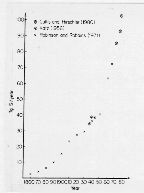 Estimated annual global sulfur emissions from
1860-1980. Source unknown.
Estimated annual global sulfur emissions from
1860-1980. Source unknown.
Sulfur emissions to the atmosphere in the US due to anthropogenic sources have also increased, as was shown in the above diagram. Emissions of sulfur per year from 1860 to 1980 in the US have risen from about 10 Tg to a peak of about 32 Tg in 1970. Environmental regulations have reduced these emissions substantially in recent years in the US and many developed countries that can afford to install sulfur emissions abatement equipment. Developing countries experiencing rapid growth or use of high- sulfur coal and low-technology combustion equipment are experiencing growing emissions.
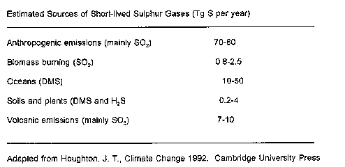 Estimated sources of
short-lived sulfur gases. Adapted from IPCC, 1992.
Estimated sources of
short-lived sulfur gases. Adapted from IPCC, 1992.
The main global source of anthropogenic sulfur is burning of high-sulfur coal, which contributes 70-80 Tg of sulfur per year, mostly in the form of sulfur dioxide (). Biomass burning contributes 0 .8 to 2.5 Tg to the global total. Natural sources include ocean production of dimethyl sulfide (DMS), soil and plant production of DMS and hydrogen sulfide (). Volcanoes, which of course are episodic sources, may contribute 7 to 10 Tg annually. This table clearly shows that anthropogenic emissions now dominate natural sources of sulfur in the atmosphere.
Sulfur compounds, like , are short-lived species in the atmosphere that are subject to chemical transformation, washout, and dry deposition and lead to acid precipitation problems. We know of sulfur dioxide as a pollutant because it reacts with water () to form sulfuric acid (). If we were able to switch off all the power plants and other anthropogenic as well as natural sources of sulfur, we could essentially eliminate sulfur from the atmosphere in a couple of weeks.
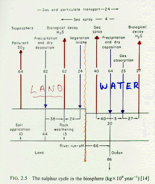 The sulfur cycle in the biosphere. J. D. Butler, Air Pollution Chemistry,
1979 .
The sulfur cycle in the biosphere. J. D. Butler, Air Pollution Chemistry,
1979 .
The sulfur cycle can be divided into a cycle over water and a cycle over land. In comparison with the nitrogen cycle, we notice immediately is that the sulfur cycle has no connection to the stratosphere, since there are no long-lived species of sulfur. Sulfur is a problem, of course in the troposphere, as an air pollutant, which we will come back to in a future learning unit.
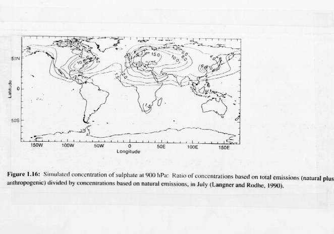 Simulated concentrations
of sulfate at 900hPa. IPCC, 1990
Simulated concentrations
of sulfate at 900hPa. IPCC, 1990
The next figure shows a simulation of sulfate () concentrations the lower atmosphere (at a level of 900 hectopascals, which is about a kilometer above the earth's surface) over the earth. The numbers plotted are dimensionless ratios of total concentration of anthropogenic plus natural sulfate divided by the concentration based on natural emissions. Highly populated and industrial areas of the eastern part of the U.S. and eastern Europe have highest concentrations. Concentrations over Asia are increasing, particularly in the industrial area of southeast China. Of course, as the Chinese industrialization rapidly increases, this problem is likely to be an increasing problem in that country.
A recent finding, and one that has put environmentalists in a perplexing dilemma, is that there also is a secondary effect of sulfur dioxide in the earth's atmosphere. Although it is not a greenhouse gas, it does contribute to the radiation balance of the earth. In the presence of clouds, atmospheric becomes dissolved in the water droplets and forms weak sulfuric acid, . Such clouds observed from space appear brighter than natural clouds, suggesting that these clouds are reflecting more solar radiation than natural clouds. This process is called cloud brightening and reduces the amount of solar energy entering the earth/atmosphere/ocean system, thereby contributing to a cooling of the planet . The net result of burning fossil fuels containing sulfur (mainly coal) is that the emitted leads to global warming and the leads to global cooling. Environmentalists have fought for years to have emissions reduced, but one result of these efforts seems to be that global warming will be exacerbated.
Another possible linkage of sulfur to global change is the role of dimethylsulfide (DMS) in formation of clouds over ocean areas. DMS is produced naturally in ocean areas by biological activity. Studies have shown that DMS can promote the production of cloud condensation nuclei, which are favored particles for cloud droplet growth. Therefore, an abundance of marine plant life can produce sufficient amounts of DMS to enhance local cloud formation and possibly increased precipitation. This constitutes a direct link between the biosphere and local meteorology. It also opens the possibility that there might be a link between changes in the stratospheric ozone and local meteorology in that, for instance, increased ultraviolet levels over the ocean could suppress ocean biology, which in turn would reduce the emission of DMS, which could reduce cloudiness and precipitation in ocean areas. We don't know enough about the magnitude of this effect to evaluate its importance in relation to other global change processes.
Several other questions relating to the sulfur cycle and its component fluxes and resevoirs indicate that much research remains to be done on this trace gas.
Phosphorus is another element that is used by plants both on land and in the ocean, and so phosphorus availability in soils and in the ocean is a regulator of biological activity. There are many unanswered questions relating to the phosphorus cycle. The mechanisms controlling the availability of phosphorus in terrestrial soils and how these mechanisms respond to processes such as acid deposition, fire, and deforestation are not well known. By these land-use practices, we might be creating imbalances in the availability of other nutrients that plants need. What is the flux of marine phosphorus to the oceans? How has it changed in the past and how is it changing today? What are the consequences of these changes? Many issues remain unanswered.
It should be apparent from these questions and from our consideration of other chemical cycles that it is not possible to consider any of these individual elements such as carbon, nitrogen, sulfur, or phosphorus alone. Plants are mainly carbon, but they need nitrogen, sulfur, and phosphorus to flourish. So a complete understanding of the carbon cycle requires an understanding of the larger system known by the term of biogeochemical cycles. Other trace gases of lesser global importance are also lumped into this general category because they may participate in the one or more of the many pathways followed by the major chemicals in their natural cycles.
Tropospheric ozone is a chemical that may be a trace constituent of natural biogeochemical cycles, but which presents an environmental problem primarily due to large anthropogenic sources in major cities. In future learning units we will discuss the problem of diminishing amounts of ozone in the stratosphere, but for now we are focusing on an excess of ozone in the lower levels in the atmosphere. Ozone is a very reactive chemical that interacts with plant and animal living tissue in a detrimental way. It can reduce lung functioning in humans and suppress plant growth enough to reduce yields of agricultural and horticultural crops.
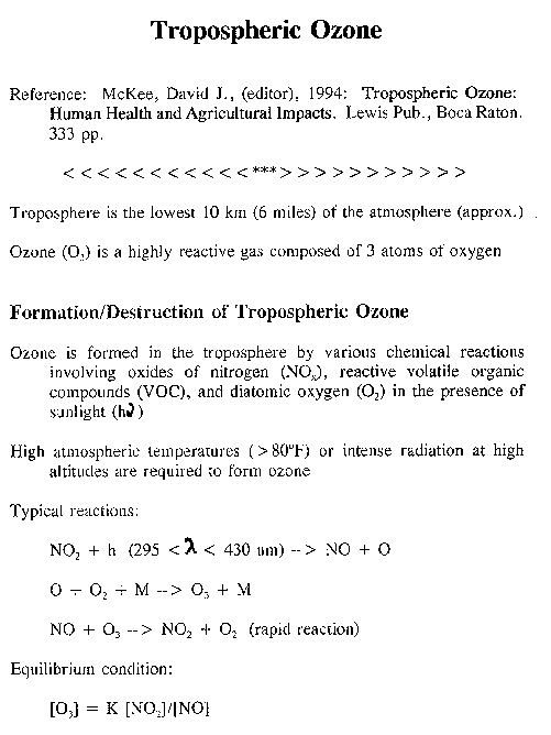 Formation/destruction of tropospheric ozone. Mckee, David J. 1994: Tropospheric
Ozone: Human Health and Agricultural Impacts. Lewis Publications, Boca Raton. 333 pp.
Formation/destruction of tropospheric ozone. Mckee, David J. 1994: Tropospheric
Ozone: Human Health and Agricultural Impacts. Lewis Publications, Boca Raton. 333 pp.
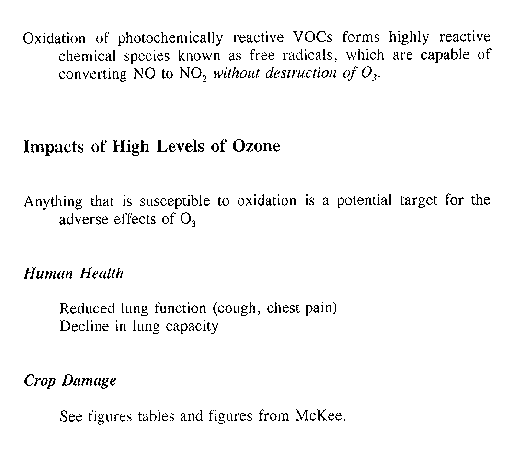 Impact of high levels of ozone. Mckee, David J. 1994:
Tropospheric
Ozone: Human Health and Agricultural Impacts. Lewis Publications, Boca
Raton. 333 pp.
Impact of high levels of ozone. Mckee, David J. 1994:
Tropospheric
Ozone: Human Health and Agricultural Impacts. Lewis Publications, Boca
Raton. 333 pp.
Ozone is formed in the troposphere by various chemical reactions involving a combination of the oxides of nitrogen, reactive volatile organic compounds (VOC) produced by a combination of exhaust from automobiles in the form of unburned hydrocarbons, and diatomic oxygen in the presence of sunlight. High atmospheric temperatures and/or intense radiation at high altitudes are required to form ozone.
Typical reactions to create ozone include nitrogen dioxide being acted upon by sunlight in the wavelength region of 295 and 430 microns to give NO plus an oxygen. The free oxygen combines with diatomic oxygen in the presence of another molecule (to give a momentum balance) to produce ozone. A rapid ozone destruction reaction consists of NO interacting with ozone to produce and . With ozone continually being produced and destroyed by these two reactions, an equilibrium condition is established in which the intermediate constituent, namely ozone, exists at a concentration determined by the ratio of the abundance of and NO. Oxidation of photochemically reactive VOCs forms highly reactive chemical species known as free radicals, which are capable of converting NO and without the destruction of . As a result, these volatile organic compounds, mainly produced by automobiles, can interfere with the natural ozone destruction process and allow ozone concentrations to become elevated.
If any one of the four ingredients (, VOC, , and sunlight) is absent, ozone concentrations diminish. Morning and evening rush-hour traffic in major cities on clear warm days provide the sufficient amounts of all ingredients, but elimination of any one reduces ozone levels significantly.
Anything that is susceptible to oxidation is a potential target for the adverse effects of elevated ozone concentrations. The human lung, for instance, particularly for people who have respiratory problems, can experience diminished functioning or reduced capacity. The accompanying tables show examples of estimated yield losses for a variety of agricultural and horticultural crops due to elevated ozone levels.
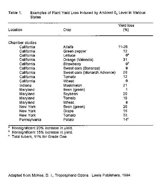 Plant yield loss due to tropospheric ozone. Adapted from McKee,
D. J., Tropospheric Ozone: Lewis Publications, 1994.
Plant yield loss due to tropospheric ozone. Adapted from McKee,
D. J., Tropospheric Ozone: Lewis Publications, 1994.
Soybeans, for instance, under an ozone concentration of .081 parts per million will experience about a 30% loss of yield. The EPA threshold standard for ozone is .12 ppm, so even at levels below the EPA standard, soybeans could suffer loss of yield.
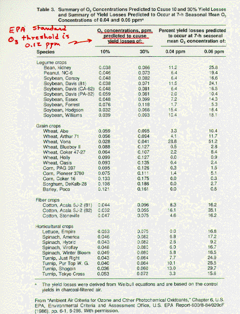 Summary of ozone concentrations
predicted to cause 10 - 30% yield losses and summary of yield losses
predicted to occur at 7-h seasonal mean ozone concentrations of 0.04 and
0.06 ppm. Adapted from McKee, David J., 1994: Tropospheric Ozone.
Summary of ozone concentrations
predicted to cause 10 - 30% yield losses and summary of yield losses
predicted to occur at 7-h seasonal mean ozone concentrations of 0.04 and
0.06 ppm. Adapted from McKee, David J., 1994: Tropospheric Ozone.
Other grain crops, such as wheat for instance, seem to be less vulnerable than soybeans. A quick scan of the vegetables listed also shows that ozone concentrations below the EPA standard will lead to significant yield reductions in all varieties.
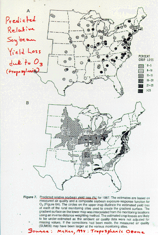 Predicted relative soybean yield
loss for 1987. McKee, David J., 1994: Tropospheric Ozone.
Figure 7, p 193. Reprinted with permission from CRC Press, Inc.
Predicted relative soybean yield
loss for 1987. McKee, David J., 1994: Tropospheric Ozone.
Figure 7, p 193. Reprinted with permission from CRC Press, Inc.
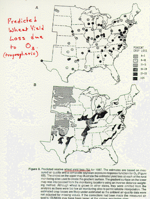 Predicted
relative wheat yield
loss for 1987. McKee, David J., 1994: Tropospheric Ozone.
Figure 7, p 193. Reprinted with permission from CRC Press, Inc.
Predicted
relative wheat yield
loss for 1987. McKee, David J., 1994: Tropospheric Ozone.
Figure 7, p 193. Reprinted with permission from CRC Press, Inc.
Transcription by Theresa M. Nichols
![]()