Enhanced Greenhouse Climate, Transient Climates

Transient Climate Simulation

The present unit describes a slightly different kind of global climate simulation, called a transient simulation. The same model is used for both equilibrium and transient simulations, but for the transient runs, external forcing (e.g., greenhouse gases, solar irradiation) are allowed to gradually change according to known (e.g, past measured greenhouse gas concentrations) or assumed future projections of external forcing. Also, internal components of the climate system (e.g., oceans, ice masses, atmosphere) are allowed to change at their natural rates in response to external forcing and feedback processes. For instance, a sudden increase in heat energy to the climate system (for whatever reason) would lead rather quickly to a rise in air temperature, but rises in land temperatures would take much longer and oceans and ice masses even longer. Similarly the gradual rate of redistribution of thermal energy (warming at the surface and cooling in the stratosphere) due to increases in greenhouse gases allows the atmosphere to keep up with these changes but the oceans and ice likely do not keep up because their time scales for change are so much longer than that of the atmosphere.

On the basis of these simple concepts we can speculate on how a transient simulation of global climate will differ from an equilibrium simulation. As greenhouse gases build up to the equivalent of twice the pre-industrial level (2xCO₂ level) in a transient simulation, the ocean and ice masses will not be in equilibrium with the rate of heating of the lower atmosphere: they will be lagging behind the rate of forcing due to their longer time scales. We can then speculate that the global-mean temperature at the time the transient simulation reached 2xCO₂ greenhouse levels would not be as high as that for an equilibrium 2xCO₂ simulated climate.

Characteristics and results of some coupled ocean-atmosphere global climate models run in transient mode are tabulated in Figure 1 for runs having various levels of increase of CO₂ (scenarios). The flux adjustment indicates how the ocean and atmosphere are coupled together. The "Warming at doubling" column gives the global mean temperature when the CO₂ passes the 2xCO₂ level (twice pre-industrial level of CO₂) in the transient run. The "Equilibrium warming" gives the global mean temperature when the model is run in equilibrium mode, and the final column gives the ratio of the previous two columns. Note that our speculation of the previous paragraph is confirmed by the last column.

GFDL Model

Recent results from the GFDL model for temperature change (Figure 2) from 1850 to 2000 show that the model is able to capture quite well the average behavior over this period. The spatial distribution of warming in the GFDL transient model (Figure 3) at the time of CO₂ doubling shows that warming is most pronounced in the polar region of the northern hemisphere. The surface warming also leads to substantial decrease in sea ice coverage over the Arctic Ocean (Figure 4). Mean sea ice thickness (in meters) in this figure is the model result for late winter and is shown for both the control and 4xCO₂ experiments.

Simulated changes in sea level Figure 5 due to thermal expansion of oceans show a 25 cm rise over 100 years and over 1 m rise in 500 years for a doubling of CO₂ as the deep ocean gradually warms in response to surface warming. Adding increased ocean water volume due to melting of ice that presently is above sea level could add substantially to sea-level rise, but these calculations currently have large uncertainty. The effect of sea-level rise on the SE and Gulf Coasts (Figure 6) of the US from the GFDL projections will first be observed in Florida and North and South Carolina.

The GFDL model has an ocean circulation component that enables us to see the effect of warming on ocean circulation Figure 7. The model simulations project global thermohaline circulation to decrease in intensity with increased greenhouse gas warming due to enhanced precipitation and runoff from the continents in high latitudes.

The GFDL model (Figure 8) projects substantial decreases in soil moisture over most mid-latitude continental areas during summer with global warming . Soil moisture reductions in major agricultural areas could negatively impact global food production as will be discussed in Unit 3-6.

Surface air temperatures (Figure 9) for a doubling of CO₂ in the GFDL model are projected to rise by about 7°C in the southeast US in July, which will significantly add to human discomfort as represented by the heat stress index (Figure 10).

The Hadley Centre Model

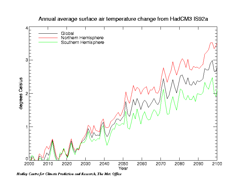
The global climate model of the Hadley Center of the United Kingdom has been used to produce maps of transient climate maps of various meteorological variables. They have simulated (Figure 12) global mean temperatures out to the year 2100. Their simulations of global patterns of temperature change also show substantial increases in the 21st century, with warming felt first in polar areas (Figure 13) but eventually spreading over most of the globe.

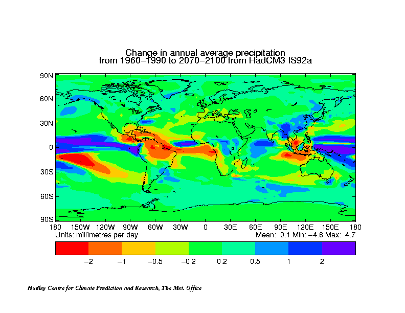
Global precipitation changes Figure 14 in the Hadley model show modest increases except in the subtropical high-pressure belts (regions of deserts) early in the 21st century. As the warming proceeds in the latter part of the 21st century, moist areas become more moist and dry areas become more dry. Rainfall in the high precipitation region of the tropical Pacific Ocean, Figure 15, we noted in Unit 1-3 becomes even more intense according to the Hadley Centre prediction. Of notable consequence is decrease in rainfall in several subtropical areas currently having limited agriculture due to water shortages, such as north and southern Africa, the Middle East, India and Australia.

Climate Simulations for the AR4

Climate model simulations for the next IPCC Assessment Report on the Impact of Climate Change to be issued in 2006 (sometimes referred to as the AR4, since it is the 4th in a series of such assessment reports by the Intergovernmental Panel on Climate Change) currently (February 2005) are being run. Equilibrium simulations, as discussed in the previous unit, give the "climate sensitivity" of the model (global mean warming in degrees C for a doubling of atmospheric CO₂). But a wider variety of transient climate runs are being made during this assessment cycle. These are listed in the following section.

Types of Transient Simulations

Pre-industrial climate: GHGs constant with time; run for 300+ years
"Climate of the 20th Century": increase GHGs each year in accordance with recorded values of the 20th Century; insert known effects of volcanoes, fluctuations in output of the sun, recorded atmospheric concentrations of sulfate aerosols, and observed changes in land use.
"Commitment runs": continue C20C through the 21st Century but with GHGs constant at current values to determine the warming we already are committed to.
Future scenario runs: Extend C20C runs into 21st Century but with various projections of growth of GHG emissions.

The goal of these more expanded runs is to provide policy makers with a wider range of information on current status of warming we have created and future impacts of alternative ways of limiting greenhouse gas emissions.

The Status of Climate Modeling

The Intergovernmental Panel on Climate Change (Houghton et al., 2001) has summarized of the status of climate modeling in its 2001 assessment of the science of climate change. The scientific consensus is that climate models generally project an increase of temperature for expected increases in greenhouse gases of from 1.5°C to 4.5°C by 2100. The spatial distribution of warming shows that land generally will warm more than oceans in the transient simulations, similar to results of equilibrium results. A minimum in the warming occurs around Antarctica and in the northern North Atlantic in the transient simulations which is related to the deep oceanic mixing in those areas as discussed in Unit 1-10 (see green hatched areas in the sketch of oceanic mixing, Figure 16 . The general tendency is for all models to show a warming, principally in late fall and winter, in high northern latitudes in connection with the reduce surface area of sea ice. The diurnal range (difference between day time maximum and night time minimum) of temperature is reduced over land in most seasons. Effects of aerosols are not uniformly distributed over the globe, but favor a reduced warming in the middle latitudes of the Northern Hemisphere (close to the sources of the aerosol). All models produce an increase in mean global precipitation and an increase in the south Asian monsoon rainfall. Models show decreased intensity of circulation in the North Atlantic ocean, principally because of increased high-latitude precipitation that reduces ocean salinity and hence suppresses deep water production in the North Atlantic (see Unit 1-10).

As of this writing (Feb 2004) one of the most recent simulations, Figure 17, of the climate of the last 140 years in comparison with the observed trend is given by transient global climate model of the National Center for Atmospheric Research reported by Wigley and available in C&E News (Hilleman, 1999) . This simulation includes the warming effect of enhanced greenhouse gas concentrations, cooling effects of sulfate aerosols, and variations due to fluctuating solar radiation. Addition of aerosols to the model has suppressed the warming as was discussed in Unit 1-12. It was pointed out in that unit that an important difference between CO₂ warming and aerosol cooling is that the longer lifetime of CO₂ means continuing emissions, even at a non-increasing rate, lead to increased radiative forcing. For aerosols, with limited lifetimes, constant emission rates simply replace the aerosol particles being washed out of the atmosphere. So the aerosol radiative forcing for emissions is constant. This fact is evident in the simulation showing the individual effects of CO₂ and aerosols. The effect of fluctuations in output of the sun apparently have settled two of the recent criticisms of global climate model simulations of the 20th century, namely that their results showed substantial warming before the CO₂ levels had a chance to build up and that the cooling of the climate between 1950 and 1970 could not be simulated. Evidently, variations in output of the sun have been a significant factor in causing these two signatures of the global mean temperature record.

View Class Images

Back to Unit Page

2-4: Enhanced Greenhouse Climate, Transient Climate Simulations